Physics Lesson 16.6.1 - Useful Mathematical Background: Integral of a function - Geometrical approach

Please provide a rating, it takes seconds and helps us to keep this resource free for all to use

★★★★★ [ 1 Votes ]

Welcome to our Physics lesson on Useful Mathematical Background: Integral of a function - Geometrical approach, this is the first lesson of our suite of physics lessons covering the topic of Ampere's Law, you can find links to the other lessons within this tutorial and access additional physics learning resources below this lesson.

Useful Mathematical Background: Integral of a function - Geometrical approach

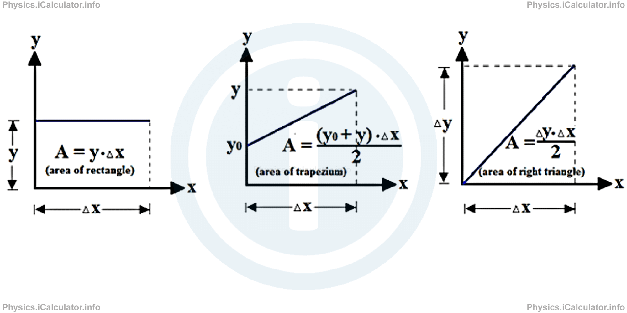
When the graph of a function has a non-complex shape - such as a straight line, parabola, trapezium and so on - the area under the graph is easy to calculate as we use known geometric formulae to find it. Look at a few examples below.

Physics Tutorials: This image provides visual information for the physics tutorial Ampere's Law

However, for more complex curves we cannot find the area under the graph that easily. In such situations, we divide the area under the graph in very small vertical strips of the same thickness Δx (more strips we have, better is) as shown in the figure below.

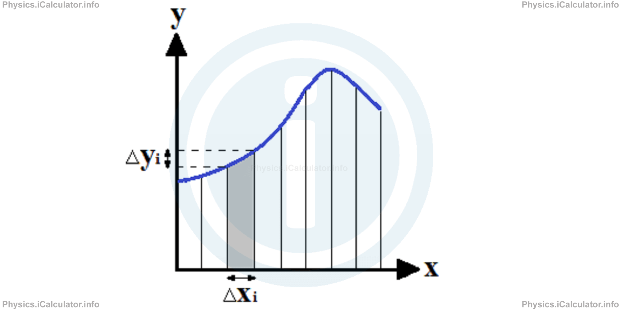
Each strip can be considered as a small trapezium of height Δx the bases of which have a difference in length of Δy. If we choose to consider one of the small trapeziums (the i-th trapezium), we obtain for its area based on the known formula:

Area of trapezium = (Longer base + Shorter base) ∙ Height/2
A_i = (y_i + y_i-1) ∙ ∆x/2

Since

y_i + y_i-1/2 = < y_i >

where < yi > is the average value of function in the i-th interval, we obtain for the area of the i-th trapezium:

A_i = < y_i > ∙ ∆x

When we want to calculate the total area under the graph, we consider all small trapeziums formed when dividing the area according the above way. Thus, we write

A_tot = ∑A_i = ∑< y_i > ∙ ∆x

Usually we write f(x) instead of y. Thus, we have for the area under the graph.

A_tot = ∑< f(x_i )> ∙ ∆x
= < f(x₁ )> ∙ ∆x + < f(x₂ )> ∙ ∆x + ⋯ + < f(x_i )> ∙ ∆x + ⋯ + < f(x_n )> ∙ ∆x

where < f(x₁) >, < f(x₂) >, < f(x_i) >, < f(x_n) >, are the average values of function in the 1st, 2nd, ith and nth trapezium respectively. (We have used the method of dividing the graph in small trapeziums when calculating the instantaneous velocity for example. In that case, we considered the slope of the graph around a given point, which corresponds to the lateral side of the small trapezium considered).

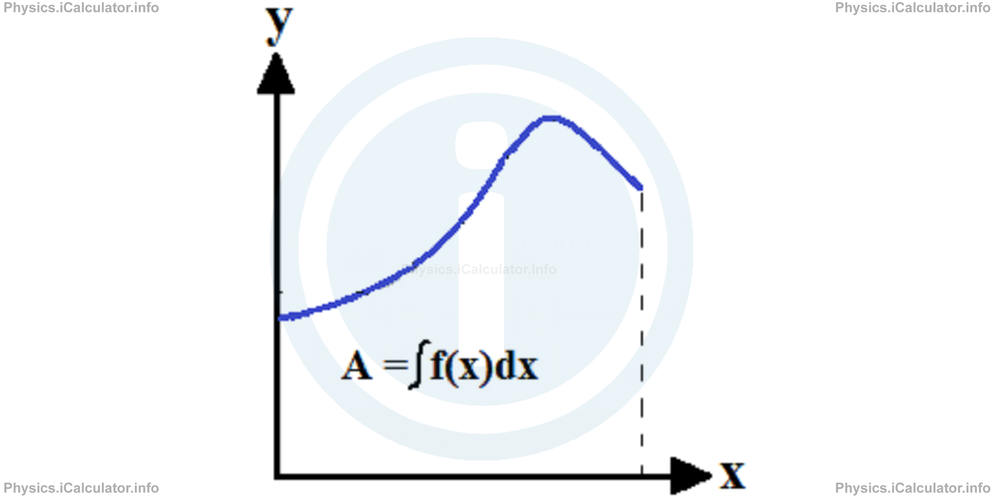
The area under the graph calculated in the above way is not 100% accurate as the graph is often a curve, not a straight line. The accuracy increases when we increase the number of divisions (the number of trapeziums therefore) so that the curve resembles more and more to a straight line (remember the Earth shape; it is curved but for small distances it looks flat). Therefore, the accuracy of the area-under-the-graph calculation would be very high if we increased the number of divisions (of small trapeziums) to infinity. In this case, we don't use anymore the symbol "Δ" to represent the width of interval but the symbol "d" instead, which is a symbol used for infinitely small intervals. Also, we use the symbol "∫" instead of "Σ" to represent the sum of all the individual areas of the small trapeziums. In this case, the average value of function fits more and more its lower and upper value in the given trapezium (trapeziums looks more and more as rectangles). Therefore, the last equation becomes

A_tot = ∫f(x)dx

The above expression is called the integral of the function f(x). Geometrically, it represents the area confined by the graph, the horizontal axis and the two vertical lines drawn from the extremities of the graph to the horizontal axis.

The small horizontal segment "dx" is known as the differential part of the integral. It represents the width of each small vertical strip (interval). In other words, dx represents the height of each small trapezium obtained through the above method.

There is a specific method to find the value of integral for a given function. It is widely discussed in mathematics textbooks, but here we will give a few examples of integrals of some ordinary functions.

1- The integral of a constant:

∫a dx = a ∙ x

where a can be aby number, including 1.

2- The integral of a power:

∫xⁿ dx = x^n-1/n-1

3- The integral of exponential function ex:

∫e^x dx = e^x

4- The integral of sine and cosine function

∫sin⁡x dx = -cos⁡x
and
∫cos⁡x dx = sin⁡x

5- The integral of 1/x:

∫1/x dx = ln⁡x

6- The integral of differential gives the function itself as they are the inverse of each other. For example:

∫d (x² ) = ∫2x dx
= 2x²/2
= x²

Some of the above integrals are used to describe magnetic properties of matter such as Ampere's law, which we will explain in the next paragraph.

You have reached the end of Physics lesson 16.6.1 Useful Mathematical Background: Integral of a function - Geometrical approach. There are 5 lessons in this physics tutorial covering Ampere's Law, you can access all the lessons from this tutorial below.

More Ampere's Law Lessons and Learning Resources

Magnetism Learning Material
Tutorial ID	Physics Tutorial Title	Revision Notes	Revision Questions
16.6	Ampere's Law
Lesson ID	Physics Lesson Title	Lesson	Video Lesson
16.6.1	Useful Mathematical Background: Integral of a function - Geometrical approach
16.6.2	Ampere's Law
16.6.3	Magnetic Field Outside a Long Straight Wire with Current
16.6.4	Magnetic Field Inside a Long Straight Wire with Current
16.6.5	Ampere's Law Applied in Solenoids and Toroids

Whats next?

Enjoy the "Useful Mathematical Background: Integral of a function - Geometrical approach" physics lesson? People who liked the "Ampere's Law lesson found the following resources useful:

Geometrical Approach Feedback. Helps other - Leave a rating for this geometrical approach (see below)
Magnetism Physics tutorial: Ampere's Law. Read the Ampere's Law physics tutorial and build your physics knowledge of Magnetism
Magnetism Revision Notes: Ampere's Law. Print the notes so you can revise the key points covered in the physics tutorial for Ampere's Law
Magnetism Practice Questions: Ampere's Law. Test and improve your knowledge of Ampere's Law with example questins and answers
Check your calculations for Magnetism questions with our excellent Magnetism calculators which contain full equations and calculations clearly displayed line by line. See the Magnetism Calculators by iCalculator™ below.
Continuing learning magnetism - read our next physics tutorial: Faraday's Law of Induction

Help others Learning Physics just like you