Menu
Physics Lesson 16.14.3 - LC Oscillations - A Quantitative Approach
Please provide a rating, it takes seconds and helps us to keep this resource free for all to use
Welcome to our Physics lesson on LC Oscillations - A Quantitative Approach, this is the third lesson of our suite of physics lessons covering the topic of Alternating Current. LC Circuits, you can find links to the other lessons within this tutorial and access additional physics learning resources below this lesson.
LC Oscillations - A Quantitative Approach
Before deriving the equations of the physical quantities involved in a LC oscillator, we must recall the concept of derivative as a rate of function's change. For example, in kinematics, the instantaneous velocity is the rate of position change in a very narrow interval, so we can write
We say, "velocity is the first derivative of position to the time". Likewise, acceleration is the first derivative of change in velocity to the time or the second derivative of the change in position to the time (derivative of derivative). We have
and so on.
In addition, we will use again the block-and-spring and LC circuit analogy to describe the quantities involved in LC oscillation systems in a more comprehensive way. For, example, we can write for the total energy of a block-and-spring system of oscillations:
= m ∙ v2/2 + k ∙ x2/2
If we ignore any friction, then the total energy is conserved and such oscillations are known as harmonic oscillations. Since the total energy does not change with time but remains constant instead, we can write
or
= m ∙ v ∙ dv/dt + k ∙ x ∙ dx/dt
= 0
Substituting v = dx/dt and dv/dt = d2x/dt2 as discussed above, we obtain
This is the fundamental equation of block-and-spring oscillator, the general solution of which (as discussed in the tutorial 11.2), is
where xmax is the amplitude of oscillations (the maximum displacement from the equilibrium position, ω is the angular frequency, x(t) is the position of the block aa a given instant and φ is the initial phase of oscillations (not necessarily the block must be at the equilibrium position initially). 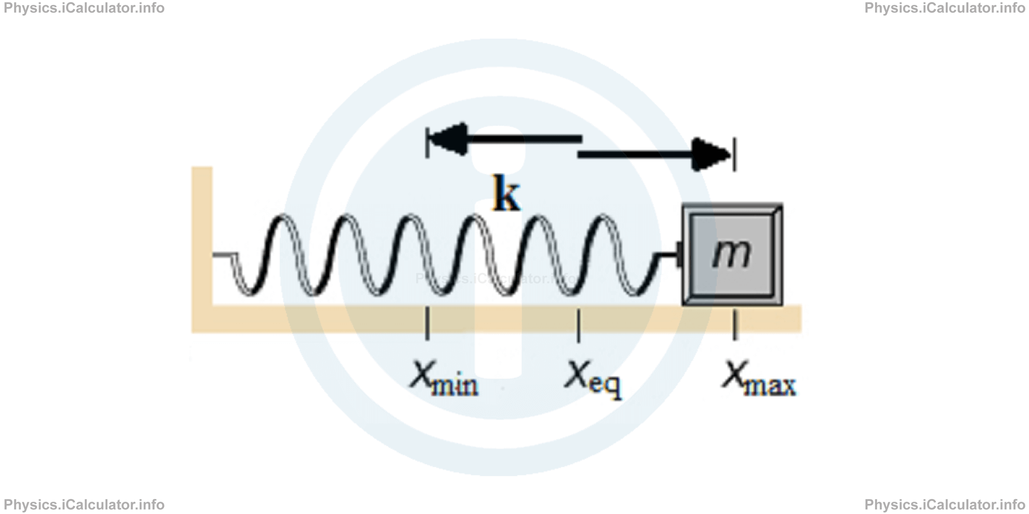
Similarly, if we substitute the above values with the corresponding ones for a LC system of oscillations given in the table of the previous paragraph, we obtain for the total energy stored in a LC system of oscillations
= L ∙ i2/2 + Q2/2C
Neglecting the resistance of the conductor, we obtain a harmonic LC oscillator in which the energy remains constant with time. Again, we can write
or
= L ∙ i ∙ di/dt + Q/C ∙ dQ/dt
= 0
Again, substituting i = dQ/dt and di/dt = d2Q/dt2, we obtain
This is the fundamental equation of a LC oscillator, the general solution of which, is
where Q(t) gives the charge stored in the capacitor at a given instant, Qmax is the maximum charge variation in the capacitor, ω is the angular frequency of LC oscillations and φ is the initial phase of oscillations.
Taking the first derivative of the last equation, we obtain the equation of current in a LC circuit. Thus,
where imax = ω ∙ t is the amplitude of the current in this kind of circuit. Hence, we can write the equation of current in a LC circuit:
Example 3
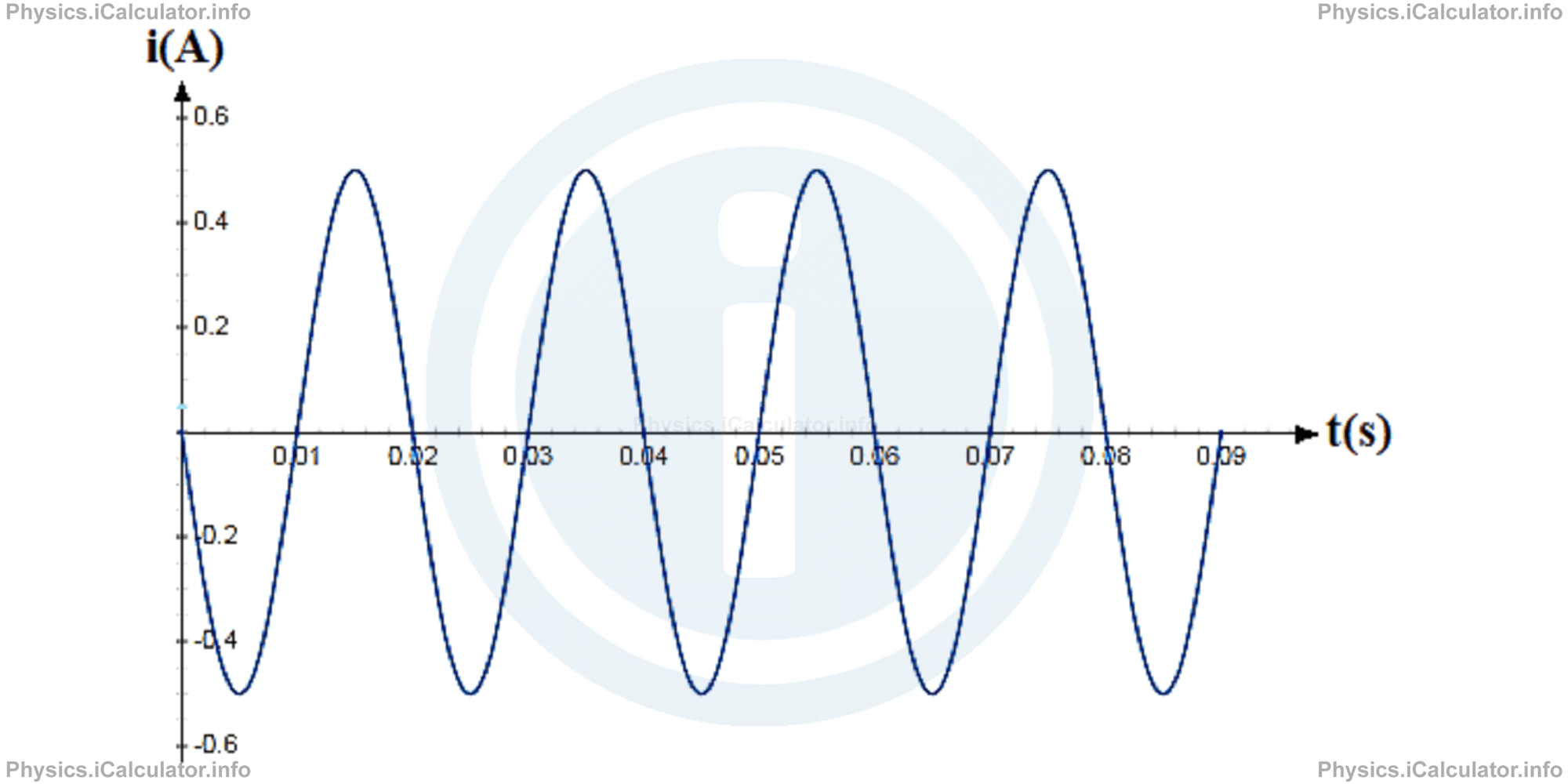
A current is flowing through a LC circuit according the sinusoidal function shown in the i vs t graph below.
Calculate:
- The frequency of current in the circuit
- The angular frequency
- The initial phase
- The equation of current in this circuit
- The current in the circuit after 2 s
- The current in the circuit after 3.079 s
Solution 3
- From the graph, we can see that one cycle is completed in 0.02 s. This value represents the period T of oscillations in the LC circuit. Since frequency f is the inverse of period, we obtain f = 1/T
= 1/0.02 s
= 50 Hz - The angular frequency ω of the LC circuit is ω = 2 ∙ π ∙ f
= 2 ∙ 3.14 ∙ 50 Hz
= 314 rad/s - From the graph we can see that the current at the beginning is zero, despite its amplitude imax is 0.5 A. Therefore, we obtain for the initial phase φ: i(t) = -imax ∙ sin(ω ∙ t + φ)Thus, sin φ must be zero to fit the values. This means φ = 0 because sin 0 = 0.
i(0) = -imax ∙ sin(ω ∙ 0 + φ)
0 = -0.5 ∙ sin(314 ∙ 0 + φ)
0 = -0.5 ∙ sinφ - The general equation of current in this LC circuit, therefore is i(t) = -(0.5 A) ∙ sin(100π ∙ t)ori(t) = -(0.5 A) ∙ sin(314 ∙ t)
- Substituting t = 2, we obtain for the current in the circuit after 2 s: i(2) = -(0.5 A) ∙ sin(100 ∙ π ∙ 2)(We know that 2π rad = 3600, so sin (N ∙ 2π) = sin 2π = sin 0 = 0. Here we have N = 100.)
= -(0.5 A) ∙ sin[100 ∙ (2π)]
= -(0.5 A) ∙ sin[100 ∙ 0]
= -(0.5 A) ∙ sin0
= 0 - We must substitute t = 3.079 in the equation of current to find the current in this instant. Thus, i(3.079) = -(0.5 A) ∙ sin (100 ∙ π ∙ 3.079)Since 306π is a multiple of 2π (306π = 153 ∙ 2π) and giving that sin 2π = 0, we write
= -(0.5 A) ∙ sin (307.9 ∙ π)
= -(0.5 A) ∙ sin (306 ∙ π + 1.9 ∙ π)i(3.079) = -(0.5 A) ∙ sin (1.9 ∙ π)
= -(0.5 A) ∙ (-0.309)
= 0.1545 A
You have reached the end of Physics lesson 16.14.3 LC Oscillations - A Quantitative Approach. There are 5 lessons in this physics tutorial covering Alternating Current. LC Circuits, you can access all the lessons from this tutorial below.
More Alternating Current. LC Circuits Lessons and Learning Resources
Whats next?
Enjoy the "LC Oscillations - A Quantitative Approach" physics lesson? People who liked the "Alternating Current. LC Circuits lesson found the following resources useful:
- Quantitative Approach Feedback. Helps other - Leave a rating for this quantitative approach (see below)
- Magnetism Physics tutorial: Alternating Current. LC Circuits. Read the Alternating Current. LC Circuits physics tutorial and build your physics knowledge of Magnetism
- Magnetism Revision Notes: Alternating Current. LC Circuits. Print the notes so you can revise the key points covered in the physics tutorial for Alternating Current. LC Circuits
- Magnetism Practice Questions: Alternating Current. LC Circuits. Test and improve your knowledge of Alternating Current. LC Circuits with example questins and answers
- Check your calculations for Magnetism questions with our excellent Magnetism calculators which contain full equations and calculations clearly displayed line by line. See the Magnetism Calculators by iCalculator™ below.
- Continuing learning magnetism - read our next physics tutorial: Introduction to RLC Circuits
Help others Learning Physics just like you
Please provide a rating, it takes seconds and helps us to keep this resource free for all to use
We hope you found this Physics lesson "Alternating Current. LC Circuits" useful. If you did it would be great if you could spare the time to rate this physics lesson (simply click on the number of stars that match your assessment of this physics learning aide) and/or share on social media, this helps us identify popular tutorials and calculators and expand our free learning resources to support our users around the world have free access to expand their knowledge of physics and other disciplines.
Magnetism Calculators by iCalculator™
- Angular Frequency Of Oscillations In Rlc Circuit Calculator
- Calculating Magnetic Field Using The Amperes Law
- Capacitive Reactance Calculator
- Current In A Rl Circuit Calculator
- Displacement Current Calculator
- Electric Charge Stored In The Capacitor Of A Rlc Circuit In Damped Oscillations Calculator
- Electric Power In A Ac Circuit Calculator
- Energy Decay As A Function Of Time In Damped Oscillations Calculator
- Energy Density Of Magnetic Field Calculator
- Energy In A Lc Circuit Calculator
- Faradays Law Calculator
- Frequency Of Oscillations In A Lc Circuit Calculator
- Impedance Calculator
- Induced Emf As A Motional Emf Calculator
- Inductive Reactance Calculator
- Lorentz Force Calculator
- Magnetic Dipole Moment Calculator
- Magnetic Field At Centre Of A Current Carrying Loop Calculator
- Magnetic Field In Terms Of Electric Field Change Calculator
- Magnetic Field Inside A Long Stretched Current Carrying Wire Calculator
- Magnetic Field Inside A Solenoid Calculator
- Magnetic Field Inside A Toroid Calculator
- Magnetic Field Produced Around A Long Current Carrying Wire
- Magnetic Flux Calculator
- Magnetic Force Acting On A Moving Charge Inside A Uniform Magnetic Field Calculator
- Magnetic Force Between Two Parallel Current Carrying Wires Calculator
- Magnetic Potential Energy Stored In An Inductor Calculator
- Output Current In A Transformer Calculator
- Phase Constant In A Rlc Circuit Calculator
- Power Factor In A Rlc Circuit Calculator
- Power Induced On A Metal Bar Moving Inside A Magnetic Field Due To An Applied Force Calculator
- Radius Of Trajectory And Period Of A Charge Moving Inside A Uniform Magnetic Field Calculator
- Self Induced Emf Calculator
- Self Inductance Calculator
- Torque Produced By A Rectangular Coil Inside A Uniform Magnetic Field Calculator
- Work Done On A Magnetic Dipole Calculator