Physics Lesson 15.5.2 - Kirchhoff's Current Law

Please provide a rating, it takes seconds and helps us to keep this resource free for all to use

★★★★★ [ 1 Votes ]

Welcome to our Physics lesson on Kirchhoff's Current Law, this is the second lesson of our suite of physics lessons covering the topic of Kirchhoff Laws, you can find links to the other lessons within this tutorial and access additional physics learning resources below this lesson.

Kirchhoff's Current Law

Circuits are not always as simple as we have seen when using Ohm's Law. In general, an electrical circuit contains more than one source distributed in many branches of the circuit. For example, a room contains a number of plugs that represents individual power sources. Also, it contains a number of series and parallel branches. We can realize the existence of parallel branches when a component such as a lamp burns out. The other components operate regularly in the circuit, which indicates the components are connected in parallel.

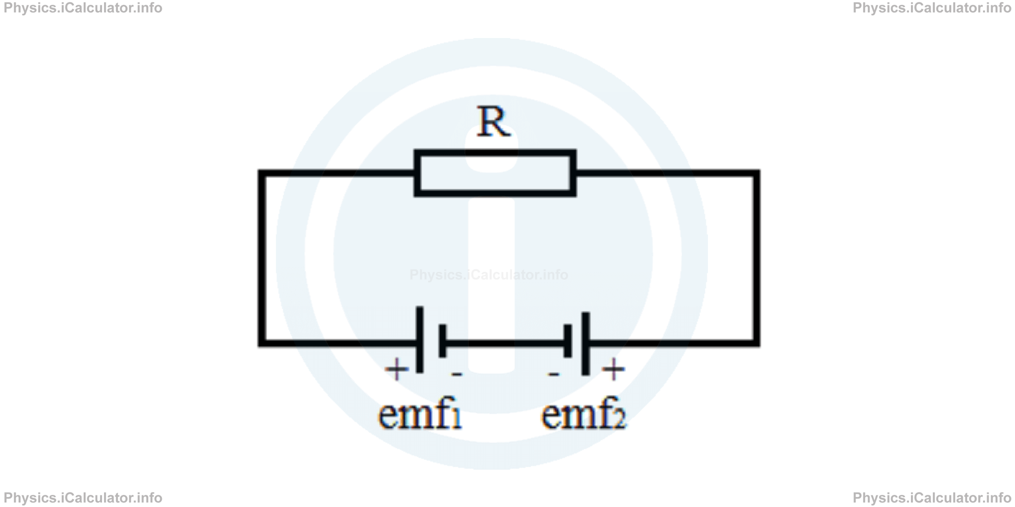
When there is an electric circuit supplied by a direct source cell or battery), there may arise an additional problem: the cells may hamper each other's work, as shown in the figure below,

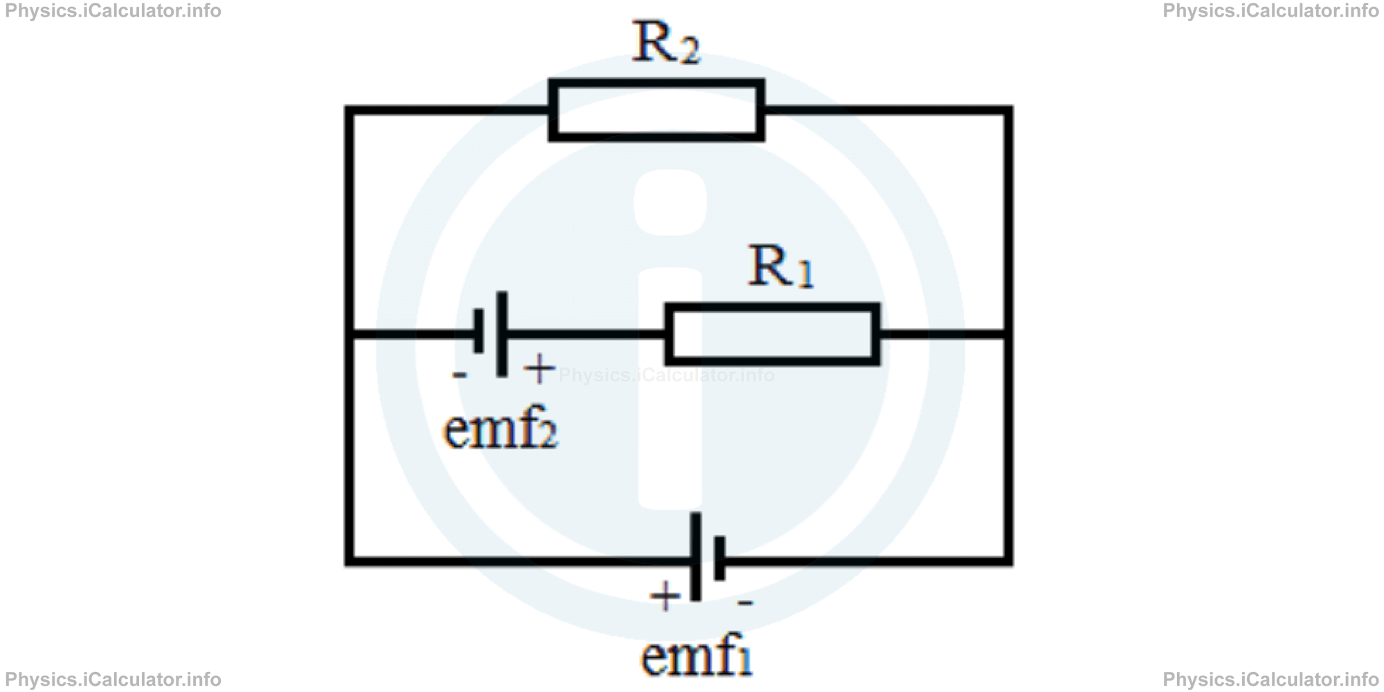
Physics Tutorials: This image provides visual information for the physics tutorial Kirchhoff Laws

or two cells may be in two different branches of the circuit, like in the figure below.

In either case, the application of Ohm's Law is impossible, as the current does not flow in a single direction. Therefore, we must apply other methods to find the missing values of circuit elements.

In 1845, Gustav Kirchhoff - a German scientist - discovered a method consisting in two laws, one for currents and the other for voltages and electromotive forces in the circuit. In this paragraph, we will discuss the first law, the Kirchhoff's Currents Law. It states that:

The sum of currents entering in a node is equal to the sum of currents leaving the node.

The mathematical equation that expresses the First Kirchhoff Law (or the Kirchhoff Law of Currents) is

I_total (in)=I_total (out)

Let's consider again the circuit discussed in the solved example of the previous paragraph in which a slight modification is made: a power source is added between R₂ and the principal node A.

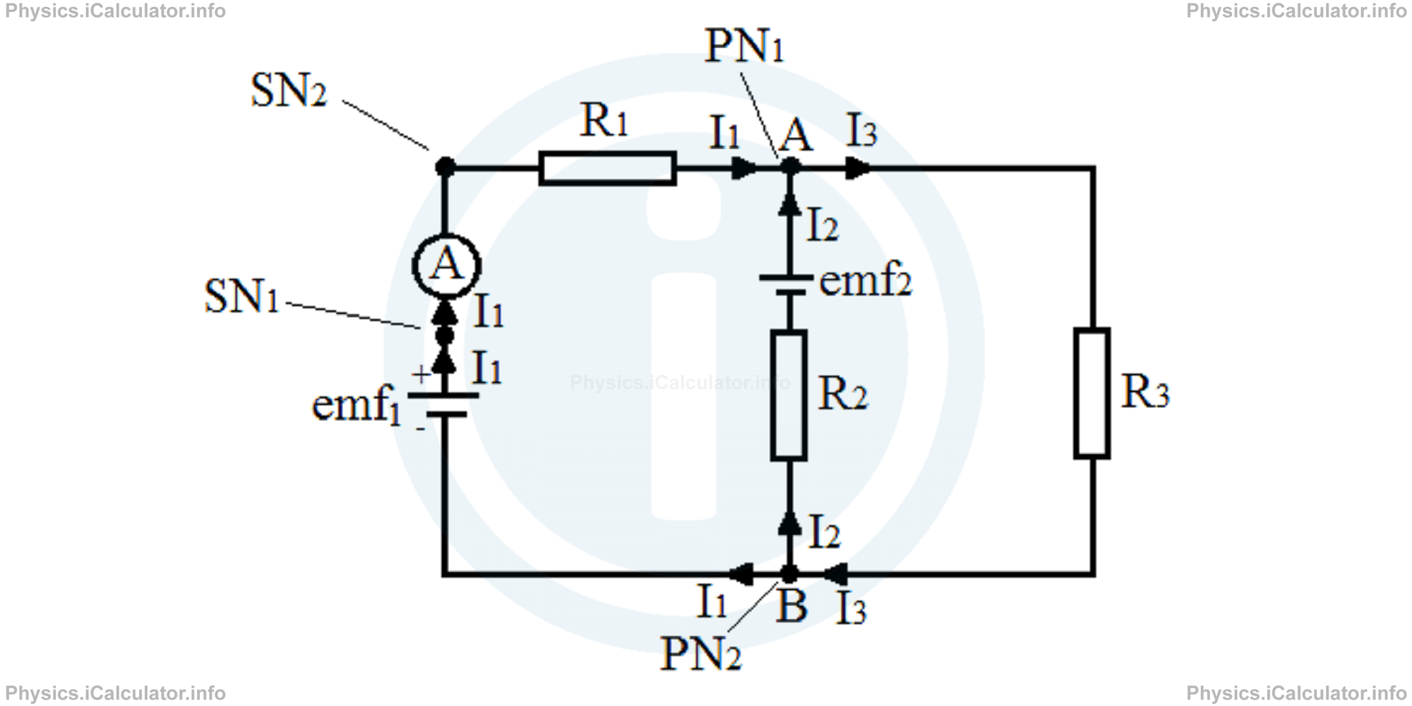
In the simple node A, there is the current I₁ that is entering the node and the same current leaving the node. Therefore, we have

I_total (in) = I_total (out)

I₁ (in SN₁ ) = I₁ (out of SN₁ )
I₁ = I₁

It is obvious the above equation is always true as when leaving the right side empty by sending I₁ on the left side, we obtain a mathematical identity of the form 0_x = 0, which is true for all values of x.

The same procedure is used to prove the correctness of the First Kirchhoff Law in the other simple nodes as well.

As for the principal nodes, we must see what happens to the currents in the points A and B of the above circuit. Thus, at the point A there are two currents entering the node (I₁ coming from the source emf₁ and I₂ coming from the source emf₂). They merge at the point A producing the current I₃ that leaves the node. Mathematically we have

I₁ + I₂ = I₃

At the point B there is one current entering the node (I₃) and two currents leaving the node (I₁ and I₂). Thus we can write

I₃ = I₁ + I₂

It is obvious that the two equations above are equivalent. We have used this rule when finding the currents in a parallel branch whose sum gives the total current flowing in the main branch of the circuit.

You have reached the end of Physics lesson 15.5.2 Kirchhoff's Current Law. There are 4 lessons in this physics tutorial covering Kirchhoff Laws, you can access all the lessons from this tutorial below.

More Kirchhoff Laws Lessons and Learning Resources

Electrodynamics Learning Material
Tutorial ID	Physics Tutorial Title	Revision Notes	Revision Questions
15.5	Kirchhoff Laws
Lesson ID	Physics Lesson Title	Lesson	Video Lesson
15.5.1	Junctions, Nodes, Paths, Branches and Loops
15.5.2	Kirchhoff's Current Law
15.5.3	Kirchhoff's Voltage Law
15.5.4	Solving Complex Circuits using the Kirchhoff Laws

Whats next?

Enjoy the "Kirchhoff's Current Law" physics lesson? People who liked the "Kirchhoff Laws lesson found the following resources useful:

Current Feedback. Helps other - Leave a rating for this current (see below)
Electrodynamics Physics tutorial: Kirchhoff Laws. Read the Kirchhoff Laws physics tutorial and build your physics knowledge of Electrodynamics
Electrodynamics Revision Notes: Kirchhoff Laws. Print the notes so you can revise the key points covered in the physics tutorial for Kirchhoff Laws
Electrodynamics Practice Questions: Kirchhoff Laws. Test and improve your knowledge of Kirchhoff Laws with example questins and answers
Check your calculations for Electrodynamics questions with our excellent Electrodynamics calculators which contain full equations and calculations clearly displayed line by line. See the Electrodynamics Calculators by iCalculator™ below.
Continuing learning electrodynamics - read our next physics tutorial: Electric Power and Efficiency

Help others Learning Physics just like you