Physics Lesson 16.15.4 - Resistive, Inductive and Capacitive Load

Please provide a rating, it takes seconds and helps us to keep this resource free for all to use

★★★★★ [ 1 Votes ]

Welcome to our Physics lesson on Resistive, Inductive and Capacitive Load, this is the fourth lesson of our suite of physics lessons covering the topic of Introduction to RLC Circuits, you can find links to the other lessons within this tutorial and access additional physics learning resources below this lesson.

Resistive, Inductive and Capacitive Load

To make the understanding of a RLC circuit more digestible, we will discuss separately three simple circuits, each of them containing only an external emf and one of the three circuit components: resistor, capacitor or inductor, which produce a load in the circuit. Let's start with the circuit that produces the resistive load.

a) Resistive Load

Let's consider a circuit containing only an alternating emf source and a resistor as shown in the figure.

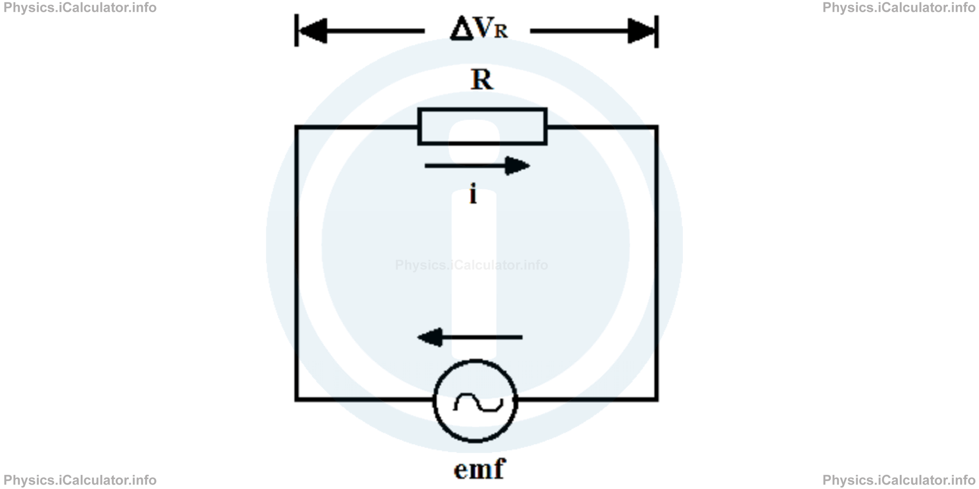
Physics Tutorials: This image provides visual information for the physics tutorial Introduction to RLC Circuits

From the Law of Energy Conservation, we have

ε - ∆V_r = 0

where ΔV_R is the potential difference across the resistor. We can write this equation as

∆V_r (t) = ε_max ∙ sin ω_d ∙ t

When neglecting the resistance of conducting wire, we obtain

i_r (t) = ε(t)/R = ε_max/R ∙ sin ω_d ∙ t

Moreover, we have for the current in the circuit:

i_r (t) = i(t) = i_max ∙ sin⁡(ω_d ∙ t-φ)

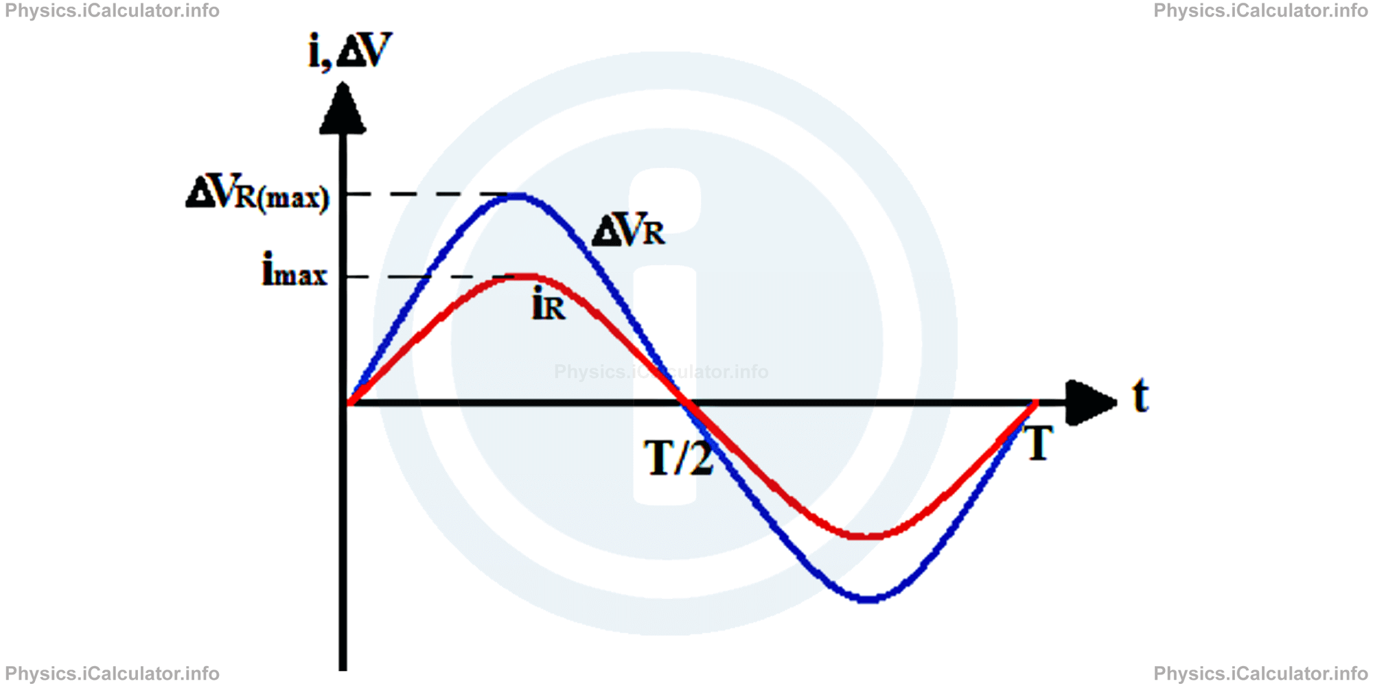
Giving that in this type of circuit the current is in phase with the potential difference, we have φ = 0. The graph below shows one cycle of induced current and potential difference in an AC circuit containing a resistive load:

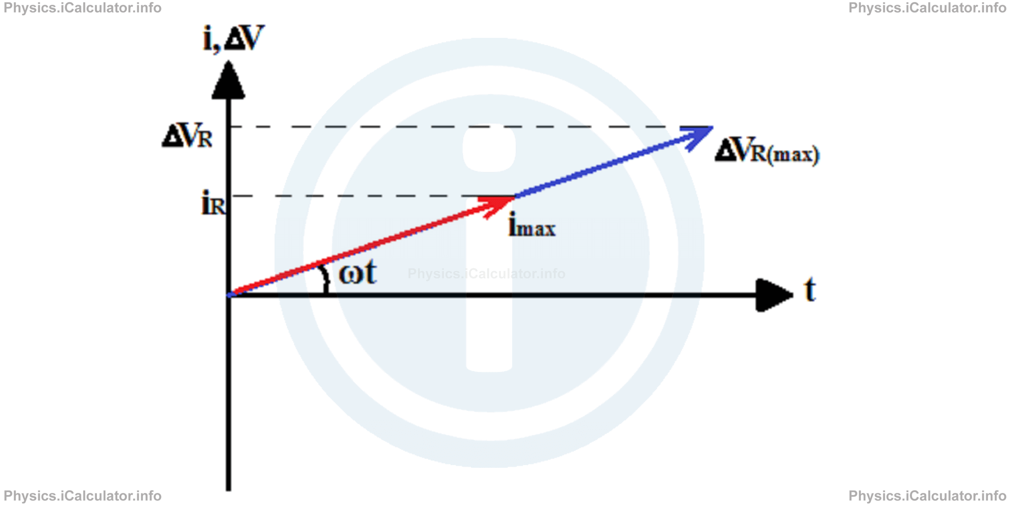
To make the graph plotting easier, we use arrows similar to vectors even though neither current nor voltage are vectors. These diagrams are known as phasor diagrams. The angle formed by the arrows and the horizontal (time) axis gives the ωt term. A phasor diagram pertaining the above graph is shown below:

Example 3

The voltage of an AC generator is given by the equation ΔV(t) = 90 sin ωt and the frequency of generator is 60 Hz. Calculate:

The maximum current produced by the generator if it is connected to a 30 Ω resistor
The potential difference in the circuit at t = 2.504 s.

Solution 3

From the equation of voltage, we notice than the maximum voltage (potential difference) in the circuit is 90 V. In addition, we obtain for the maximum current flowing through the circuit:
i_max = ∆V_max/R
= 90 V/30 Ω
= 3A
The potential difference at t = 2.504 s (giving that ω = 2πf and f = 60 Hz), is
ΔV(2.504) = 90 ∙ sin (2π ∙ 60 ∙ 2.504)
= 90 ∙ sin (2π ∙ 60 ∙ 2.504)
= 90 ∙ sin 300.48π
= 90 ∙ sin 0.48π
= 90V ∙ 0.998
= 89.82 V

b) Capacitive Load

Now, let's consider a circuit supplied by an AC source, which contains only a capacitor C as shown in the figure.

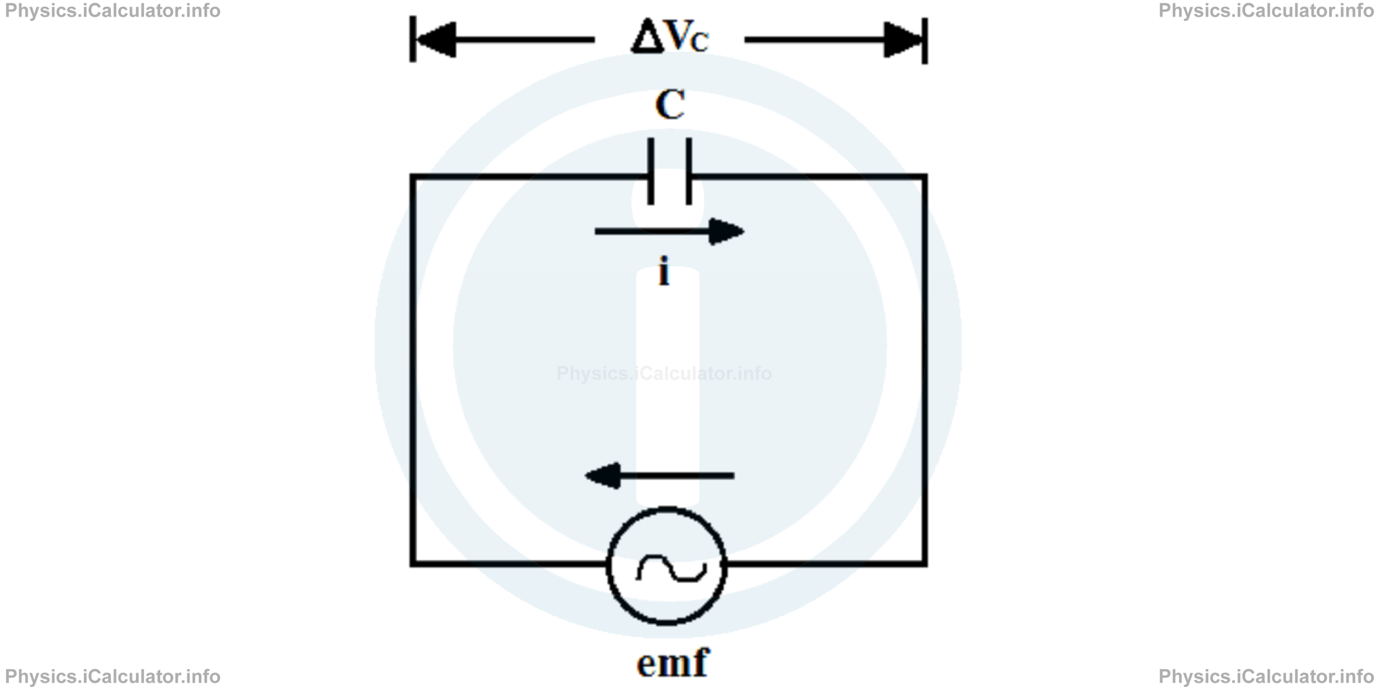
Using a similar approach as we did when dealing with the resistive load, we obtain for the potential difference at any instant across the capacitor:

∆V_c (t) = ∆V_C(max) ∙ sin⁡ω_d ∙ t

From the definition of capacitance, we have for the charge stored in the capacitor at any instant t:

Q_c (t) = C ∙ ∆V_c (t)
= C ∙ ∆V_C(max) ∙ sin ω_d ∙ t

and for the current at any instant t:

i_c (t) = dQ_c/dt = ω_d ∙ ∆V_C(max) ∙ cos ω_d ∙ t

The quantity

X_c = 1/ω_d ∙ C

is called capacitive reactance of capacitor. It has the unit of resistance (Ohm).

From experiments, it results that current leads by one quarter of a cycle the voltage in such a circuit. If we replace the cos ωd ∙ t term with a phase-shifted sine expression of + π/2 rad, we obtain

cos⁡ω_d ∙ t = sin⁡(ω_d ∙ t + π/2)

Hence, we obtain for the current in the circuit:

i_c (t) = ∆V_C(max)/X_c ∙ sin⁡(ω_d ∙ t + π/2)

In addition, we have for the maximum potential difference in the circuit

∆V_C(max) = i_C(max) ∙ X_c

Since there is a shift in phase by one quarter of a period (π/2 = 2π/4 = T/4), the graphs of potential difference and current versus time for one complete cycle are:

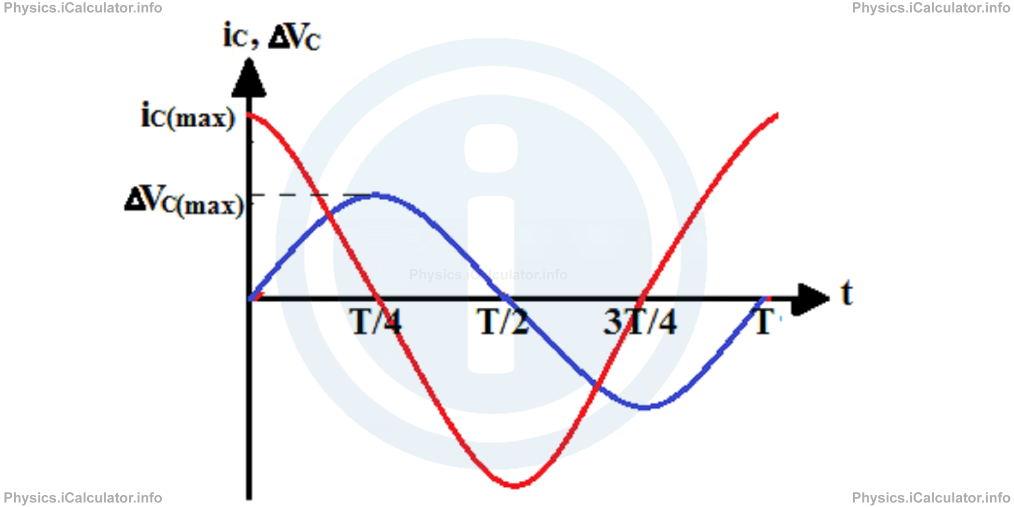
The corresponding phasor diagram for this circuit is 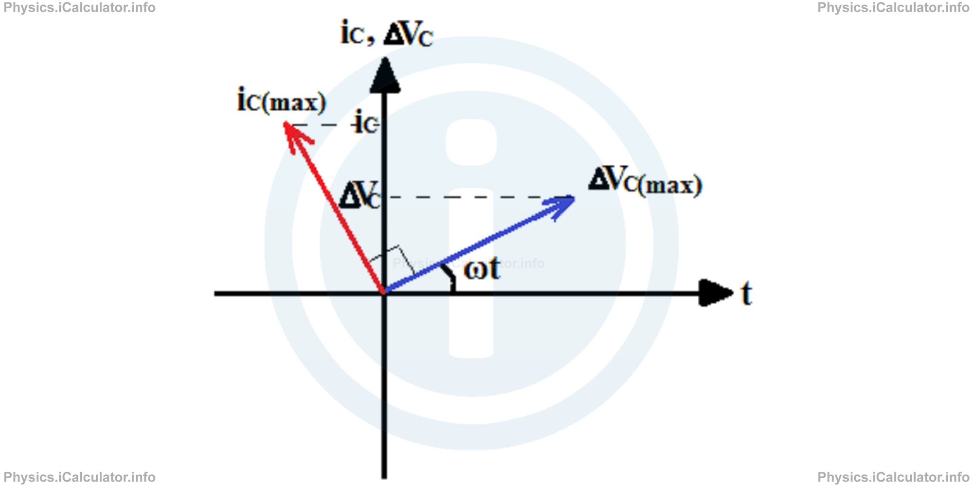Physics Tutorials: This image provides visual information for the physics tutorial Introduction to RLC Circuits

The current is π/2 (a quarter of a cycle) in advantage to potential difference. Therefore, we say: "the current leads the voltage by π/2".

Remark! The capacitive reactance behaves as an AC resistance. As the frequency of current approaches zero, the capacitive reactance raises to infinity and as a result, the circuit behaves as a DC circuit. However, the current flow in this way (in one direction only) is prevented from the high resistance between the plates of capacitor (at the gap between the plates), which does not allow the current to flow between the plates and to close therefore the cycle.

Example 4

A circuit containing a 60 Hz AC power source that oscillates according the equation ΔVC(t) = 50 ∙ sin ωd ∙ t and a 20 μF capacitor as shown in the figure.

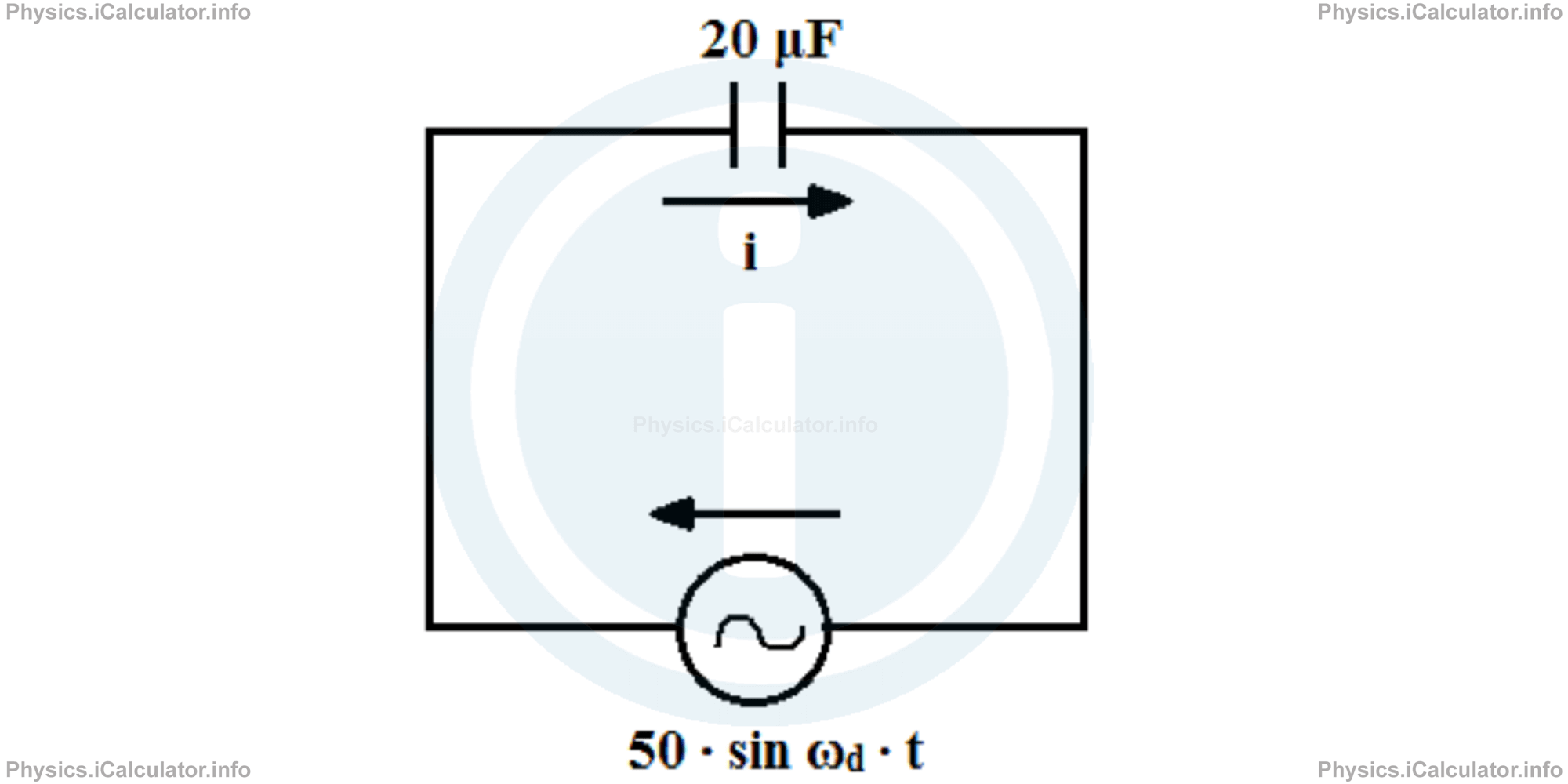
Calculate:

The capacitive reactance in the circuit
The maximum current flowing in the circuit
The value of voltage and current in the circuit at t = 1.406 s.

Solution 4

From the clues, it is clear that ΔV_C(max) = 50 V, C = 20μF = 2 × 10-5 F and f = 60 Hz. Thus, for capacitive reactance, we have
X_c = 1/ω_d ∙ C
= 1/2π ∙ f ∙ C
= 1/2 ∙ 3.14 ∙ (60 Hz) ∙ (2 × 10^-5 F)
= 132.7Ω
The maximum current flowing through the circuit is given by
∆V_C(max) = i_C(max) ∙ X_c
Thus,
i_c(max) = ∆V_c(max)/X_c
= 50 V/132.7Ω
= 0.38 A
The value of voltage in the circuit at t = 1.406 s is
∆V_c (t) = ∆V_C(max) ∙ sin ω_d ∙ t
∆V_c (1.406) = 50 ∙ sin (2π ∙ 60 ∙ 1.406)
= 50 ∙ sin (168.72π)
= 50 ∙ sin (0.72π)
= 50V ∙ 0.77
= 38.5 V
As for the current at t = 1.406 s, we have
i_c (t) = i_C(max) ∙ sin (ω_d ∙ t + π/2)
i_c (1.406) = 0.38 ∙ sin (168.72π + π/2)
= 0.38 ∙ sin (169.22π)
= 0.38 ∙ sin (1.22π)
= 0.38A ∙ (-0.64)
= -0.24 A
The negative sign shows direction; it means the current actually is flowing in the opposite direction to the initial current at t = 0.

c) Inductive Load

The reasoning is the same even when we have a circuit in which there is only an AC source and an inductor as shown in the figure.

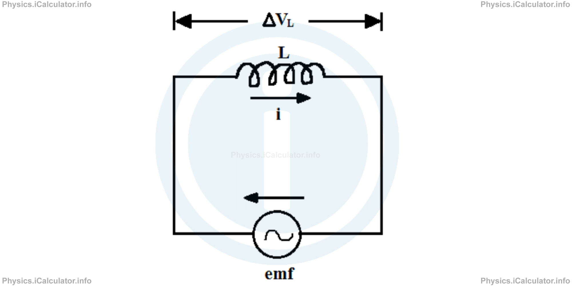
The potential difference across the inductor is

∆V_L (t) = ∆V_L(max) ∙ sin ω_d ∙ t

From Faraday's Law, we have

∆V_L = L di_L/dt

Thus, combining the above equations, we obtain

di_L/dt = ∆V_L/L = ∆V_L(max)/L ∙ sin ω_d ∙ t

di_L = ∆V_L(max)/L ∙ sin (ω_d ∙ t)dt

The current flowing at any instant in the circuit is obtained through integration techniques. Thus,

i_L (t) = ∫di_L = ∆V_L(max)/L ∙ ∫sin⁡(ω_d ∙ t)dt
= ∆V_L(max)/L ∙ (-1/ω_d ) ∙ cos⁡(ω_d ∙ t)
= -∆V_L(max)/ω_d ∙ L ∙ cos⁡(ω_d ∙ t)

The quantity

X_L = ω_d ∙ L

is called inductive reactance and is measured in Ohms, similarly to capacitive reactance discussed in the previous paragraph.

Using the trigonometric identity

-cos (ω_d ∙ t) = sin (ω_d ∙ t - π/2)

we obtain for the current flowing in a circuit containing an inductive load:

i_L (t) = ∆V_L(max)/ω_d ∙ L ∙ sin (ω_d ∙ t - π/2)

From this equation, we can see that for a purely inductive load, the current is delayed (is out of phase) by π/2 (a quarter of a cycle) to the potential difference. Therefore, we obtain the graph below:

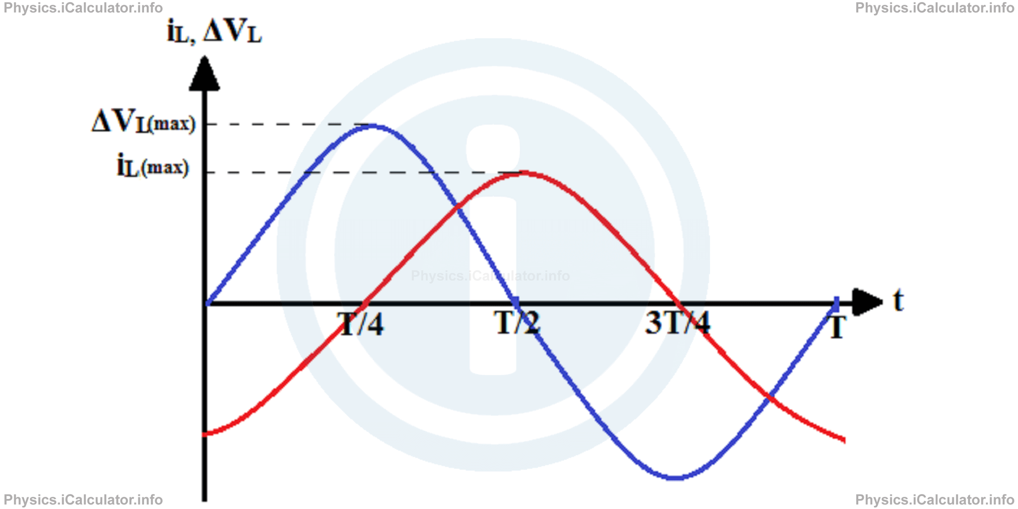
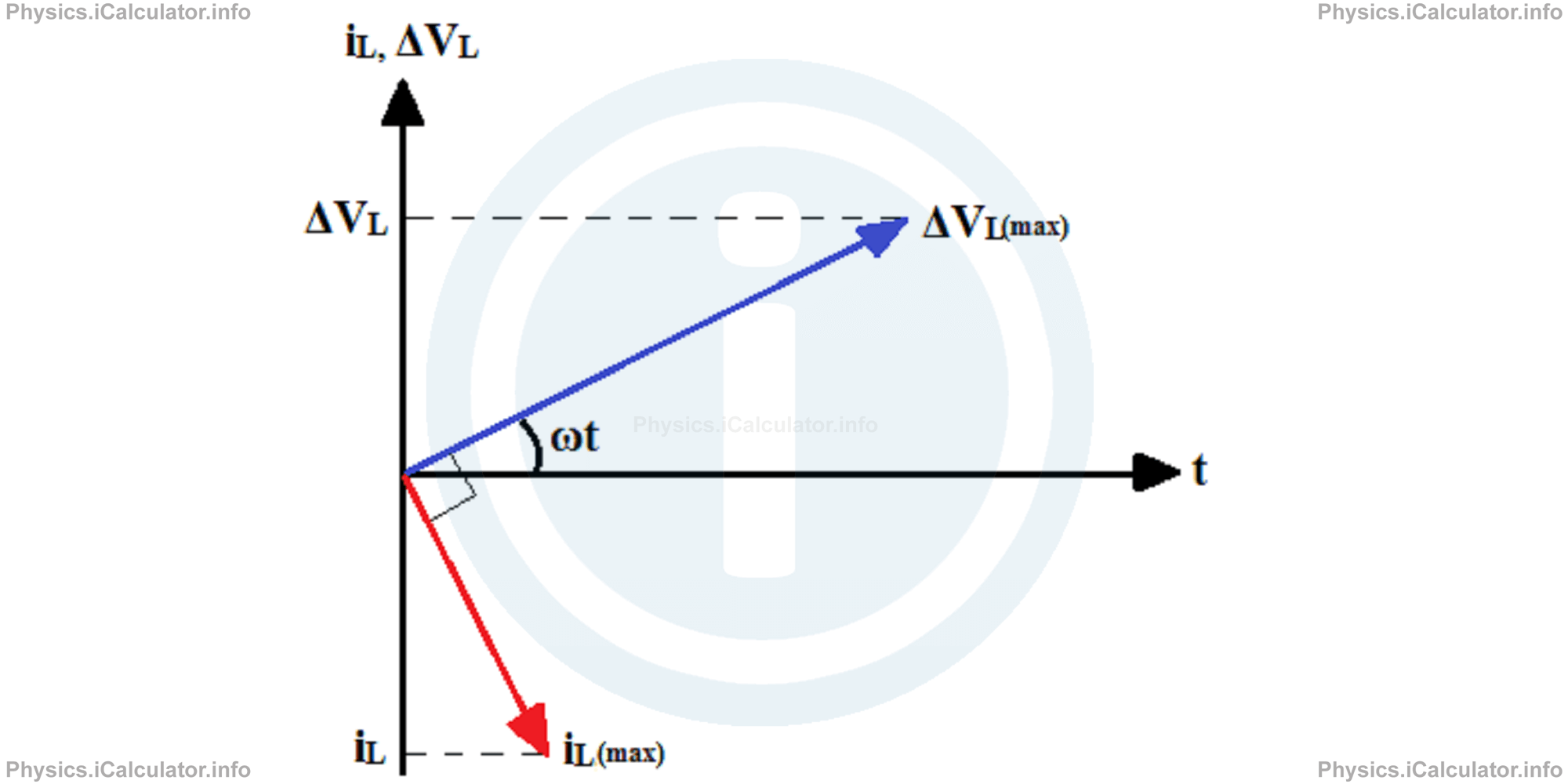
Again, we use the phasor concept to simplify the understanding of the above graph. The phasor diagram that corresponds the above graph is shown below:

Example 5

A 0.2 H inductor is connected to an AC source of voltage ΔVC(t) = 40 ∙ sin(100 π ∙ t).

Calculate the inductive reactance of the circuit
Write the equation of current in the circuit as a function of time
Calculate the current and voltage in the circuit at t = 4.961 s.

Solution 5

From the clues, we have ΔV_L(max) = 40 V and L = 0.2 H. In addition, we have
ω_d = 2πf = 100π
so, f = 50 Hz. The inductive reactance in the circuit is
X_L = ω_d ∙ L
= 100π ∙ 0.2
= 20π Ω
= 20 ∙ 3.14 Ω
= 62.8 Ω
Since the inductive reactance is like a resistance in the circuit, we obtain for the maximum current flowing through the circuit (applying the Ohm's Law):
i_L(max) = ΔV_L(max)/X_L
= 40V/62.8Ω
= 0.64A
Therefore, the equation of current in the circuit is
i_L (t) = ∆V_L(max)/ω_d ∙ L ∙ sin⁡(ω_d ∙ t - π/2)
= 40/100π ∙ 0.2 ∙ sin (100π ∙ t - π/2)
= - 2/π ∙ sin (100π ∙ t - π/2)
= 0.64 ∙ sin (100π ∙ t - π/2)
The current at t = 4.961s is
i_L (4.961) = 0.64 ∙ sin (100π ∙ 4.961 - π/2)
= 0.64 ∙ sin (100π ∙ 4.961 - π/2)
= 0.64 ∙ sin (496.1π - π/2)
= 0.64 ∙ sin (495.6π)
= 0.64 ∙ sin (1.6π)
= 0.64A ∙ (-0.95)
= 0.61A
and the voltage in the circuit at t = 4.961s is
∆V_L (t) = ∆V_L(max) ∙ sin⁡(ω_d ∙ t)
∆V_L (4.961) = ∆V_L(max) ∙ sin⁡(ω_d ∙ t)
= 40 ∙ sin⁡(100π ∙ 4.961)
= 40 ∙ sin⁡(496.1π)
= 40 ∙ sin⁡(0.1π)
= 40V ∙ 0.31
= 12.4V

You have reached the end of Physics lesson 16.15.4 Resistive, Inductive and Capacitive Load. There are 4 lessons in this physics tutorial covering Introduction to RLC Circuits, you can access all the lessons from this tutorial below.

More Introduction to RLC Circuits Lessons and Learning Resources

Magnetism Learning Material
Tutorial ID	Physics Tutorial Title	Revision Notes	Revision Questions
16.15	Introduction to RLC Circuits
Lesson ID	Physics Lesson Title	Lesson	Video Lesson
16.15.1	What is a RLC Circuit? Damped Oscillations in a RLC Circuit
16.15.2	Equation of the Damped Oscillations in a RLC Circuit
16.15.3	Forced Oscillations. Alternating Current and Emf in a RLC Circuit caused by Forced Oscillations
16.15.4	Resistive, Inductive and Capacitive Load

Whats next?

Enjoy the "Resistive, Inductive and Capacitive Load" physics lesson? People who liked the "Introduction to RLC Circuits lesson found the following resources useful:

Resistance Feedback. Helps other - Leave a rating for this resistance (see below)
Magnetism Physics tutorial: Introduction to RLC Circuits. Read the Introduction to RLC Circuits physics tutorial and build your physics knowledge of Magnetism
Magnetism Revision Notes: Introduction to RLC Circuits. Print the notes so you can revise the key points covered in the physics tutorial for Introduction to RLC Circuits
Magnetism Practice Questions: Introduction to RLC Circuits. Test and improve your knowledge of Introduction to RLC Circuits with example questins and answers
Check your calculations for Magnetism questions with our excellent Magnetism calculators which contain full equations and calculations clearly displayed line by line. See the Magnetism Calculators by iCalculator™ below.
Continuing learning magnetism - read our next physics tutorial: The Series RLC Circuit

Help others Learning Physics just like you