Physics Lesson 18.2.1 - Parametric Equations in Galilean Transformations

Please provide a rating, it takes seconds and helps us to keep this resource free for all to use

Welcome to our Physics lesson on Parametric Equations in Galilean Transformations, this is the first lesson of our suite of physics lessons covering the topic of Classical Principle of Relativity, you can find links to the other lessons within this tutorial and access additional physics learning resources below this lesson.

Parametric Equations in Galilean Transformations

Let's suppose there is an observer at rest, who is recording all events occurring in an inertial reference frame S. The origin O of space coordinates and the directions of the three axes X, Y and Z are all known. Using the standard methods, the observer associated to this inertial system measures the coordinates of any point of space. More precisely, he measures the space coordinates (x, y, z) of a material point which can be either at rest or at random motion in this inertial system.

From geometry, it is known that the 3-dimensional space is Euclidian. This means the distance of a point P(x, y, z) from origin O, is calculated through the Pythagorean Theorem.

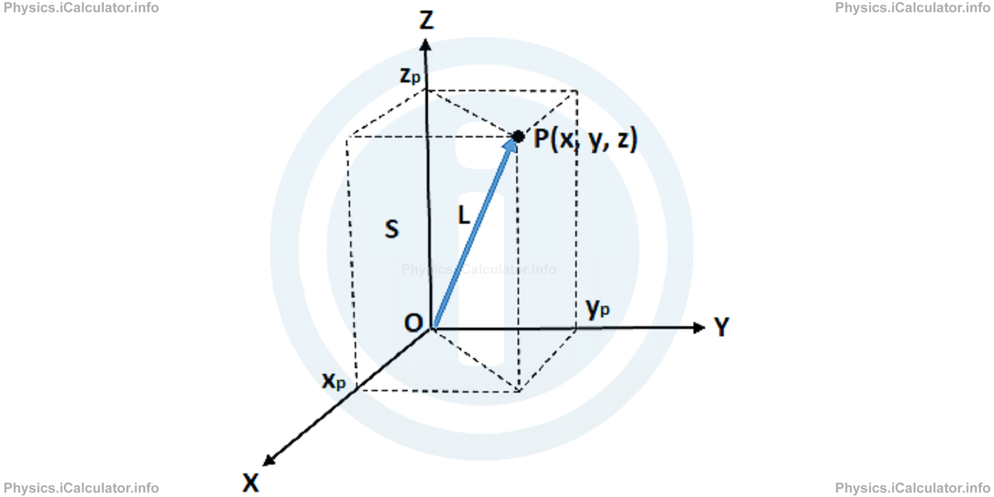
As you see from the figure, L is the diagonal of the cuboid formed by projections of the point P on each axis and the point P itself. Hence, we can write:

In addition, the observer at rest in S measures the time elapsed through a standard clock. As discussed in the previous tutorial, the time is equal and absolute for all inertial frames of reference. Principally, we assume the observer as able to measure the time through a rigorously periodical process. We denote this time by t and take its origin (t = 0) at any instant, because time is homogenous.

From mathematics, it is known that a parametric equation define a group of quantities as functions of one or more independent variables called parameters. In our case, the time t is the parameter, so we can write general form of the parametric equations of motion as

where x, y and z are the coordinates of the point P at any instant t. Obviously, we know the object's motion when we know all the above three parametric functions at any given instant.

The diagonal L of the cuboid discussed above is usually denoted by r⃗ when expressed as a vector. It is known as position vector.

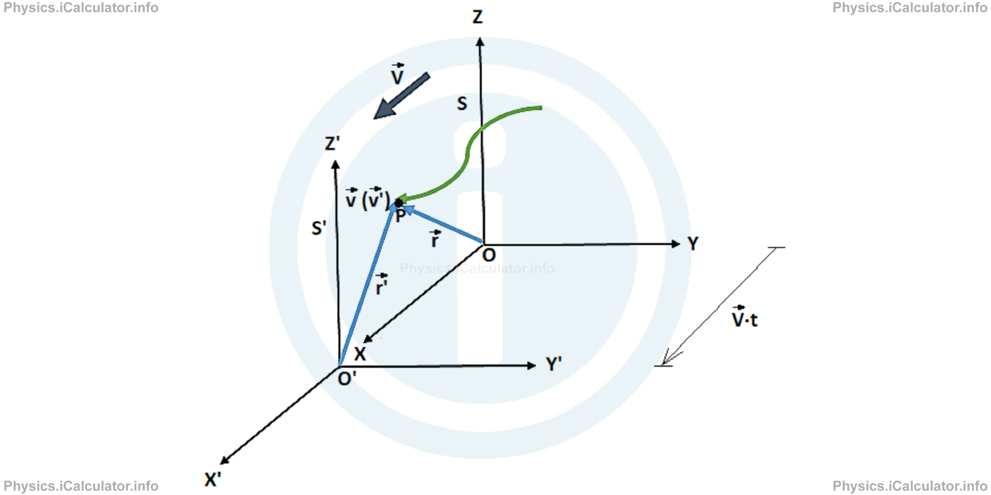
Now, let's consider the random motion of a particle P in a system S related to the Earth (i.e. we assume it as not moveable). The particle's trajectory is shown in the figure below. Then, we observe the same particle from another inertial reference system S'. Just we make sure (for convenience) to take the motion of the system S' in the X-direction of S. Obviously, the system S' moves at constant velocity V⃗ in respect to the fixed system S (as S' is inertial).

Let's take as t = 0 the instant in which the origins of the two system converge. It is clear that after a certain time t, the system S' is displaced by

in the positive direction of the X-axis. Therefore, at a given instant t, the particle P will be somewhere in the space and it will have a position vector r⃗ in the system S and r⃗' in the system S'.

From properties of vectors, is clear that:

For example, the system S' could have been connected to a train moving at constant velocity in respect to the ground. In the above figure, we also have denoted by v⃗ and v⃗' the instantaneous velocity of particle in the systems S and S' respectively.

Remark! Do not confuse the moving velocity V⃗ of the inertial reference frame S' in respect to the reference frame S (which is considered at rest) with the velocity of particle (v⃗ or v⃗') which represents the velocity of particle in the system S or S'. The first is denoted by an uppercase while the later with lowercase.

Giving that the three components of velocity vector V⃗ are (V, 0, 0), we obtain for the parametric equations of the point P in the system S' in respect to the system S:

When adding the time t as the fourth parameter and giving that t' = t in all inertial frames of reference, we obtain

These equations are nothing else but the equations of Galilean Transformations of Coordinates we obtained in the previous tutorial.

You have reached the end of Physics lesson 18.2.1 Parametric Equations in Galilean Transformations. There are 5 lessons in this physics tutorial covering Classical Principle of Relativity, you can access all the lessons from this tutorial below.

More Classical Principle of Relativity Lessons and Learning Resources

Whats next?

Enjoy the "Parametric Equations in Galilean Transformations" physics lesson? People who liked the "Classical Principle of Relativity lesson found the following resources useful:

1. Parametric Equations Feedback. Helps other - Leave a rating for this parametric equations (see below)
2. Relativity Physics tutorial: Classical Principle of Relativity. Read the Classical Principle of Relativity physics tutorial and build your physics knowledge of Relativity
3. Relativity Revision Notes: Classical Principle of Relativity. Print the notes so you can revise the key points covered in the physics tutorial for Classical Principle of Relativity
4. Relativity Practice Questions: Classical Principle of Relativity. Test and improve your knowledge of Classical Principle of Relativity with example questins and answers
5. Check your calculations for Relativity questions with our excellent Relativity calculators which contain full equations and calculations clearly displayed line by line. See the Relativity Calculators by iCalculator™ below.
6. Continuing learning relativity - read our next physics tutorial: Space and Time in Einstein Theory of Relativity

Help others Learning Physics just like you

Please provide a rating, it takes seconds and helps us to keep this resource free for all to use

We hope you found this Physics lesson "Classical Principle of Relativity" useful. If you did it would be great if you could spare the time to rate this physics lesson (simply click on the number of stars that match your assessment of this physics learning aide) and/or share on social media, this helps us identify popular tutorials and calculators and expand our free learning resources to support our users around the world have free access to expand their knowledge of physics and other disciplines.

Relativity Calculators by iCalculator™

• Energy Calculator In Relativistic Events
• Frequency Calculator During Doppler Effect In Relativistic Events
• Length Calculator In Relativistic Events
• Lorentz Transformation Of Coordinates Calculator
• Lorentz Transformation Of Velocity Calculator
• Mass And Impulse Calculator In Relativistic Events
• Time Calculator In Relativistic Events
• Velocity Calculator In Relativistic Events