Physics Lesson 3.11.5 - What happens if the acceleration is not constant?

Please provide a rating, it takes seconds and helps us to keep this resource free for all to use

★★★★★ [ 1 Votes ]

Welcome to our Physics lesson on What happens if the acceleration is not constant?, this is the fifth lesson of our suite of physics lessons covering the topic of Acceleration v's Time Graph, you can find links to the other lessons within this tutorial and access additional physics learning resources below this lesson.

What happens if the acceleration is not constant?

In this case, we cannot use anymore the five Equations of Motion (the equation of uniform motion and the four equations of motion with constant acceleration. Therefore, we need to find other ways to solve the problems involving motions with non-constant acceleration. We have two cases in this regard:

a. When acceleration changes uniformly

In this case, we can make use of the average acceleration concept and then consider the process as a motion with constant acceleration (where this constant acceleration is represented by the value of average acceleration) as shown in the graph below.

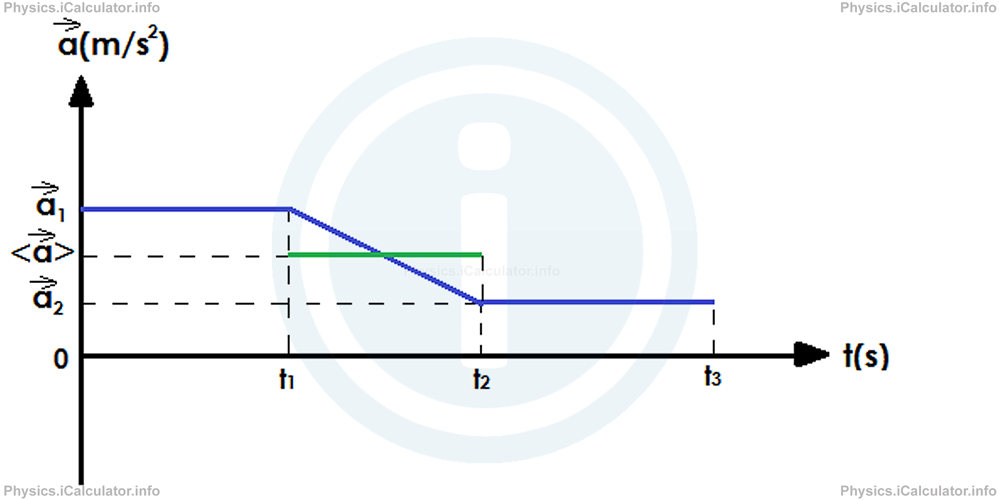
From the figure we can see the acceleration is constant during the first and the third intervals. It is a⃗₁ and a⃗₂ respectively during the abovementioned intervals.

In the second interval, the acceleration decreases uniformly. Therefore, we can use the concept of average acceleration < a⃗ > to make possible using the kinematic formulae in this interval. Since the acceleration changes uniformly, we can write for the acceleration in the second interval

< a⃗ > = a⃗₁+a⃗₂/2

Like in the other graphs, we can use the concept of area under the graph to express other kinematic quantities. Thus,

"The area under the acceleration vs time graph represents the change in velocity"

Example 3

The acceleration vs time graph of a moving object is shown in the figure below.

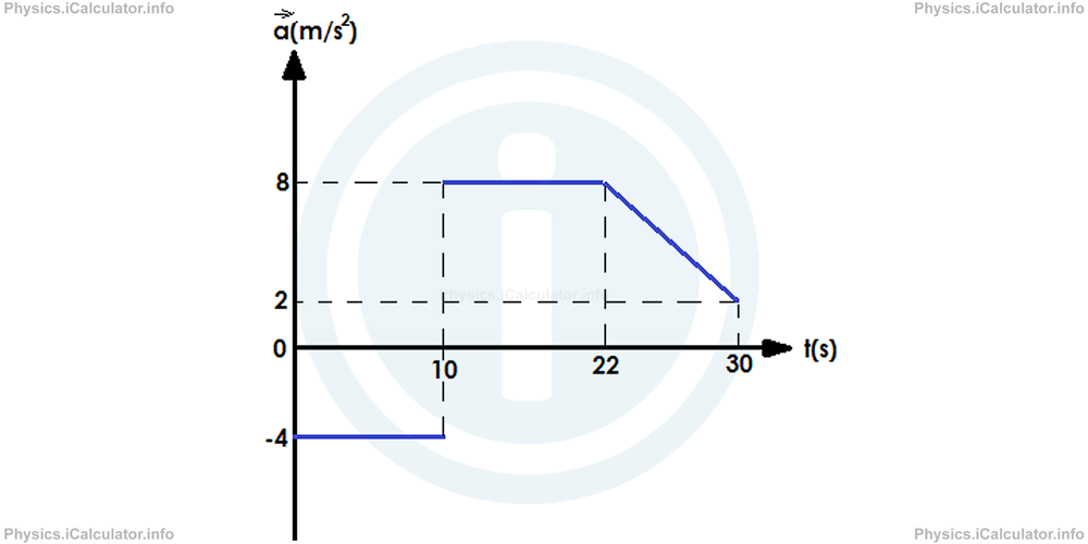
The object is initially moving at 40 m/s.

Calculate:

The velocity at t₁ = 10s, t₂ = 22s and t₃ = 30s
The displacement in each interval
The total displacement of the object
The average velocity of the entire motion

Solution 3

1. We can use the equation v⃗ = v⃗₀ + a⃗ × t to find the velocities at each of the instants required. Thus, since the acceleration in the first interval is a⃗₁ = -4 m/s², we have

v⃗₁ = v⃗₀ + a⃗₁ × t₁
= 40 + (-4) × 10
= 40 - 40
= 0

In the second interval, we have a⃗₂ = 8 m/s². Also, the time interval t₂ is 22s - 10s = 12s. Thus, the velocity at the end of this interval is

v⃗₂ = v⃗₁ + a⃗₂ × t₂
= 0 + 8 × 12
= 96 m/s

In the third interval, the acceleration is not constant. It decreases uniformly from a⃗₂ = 8 m/s² to a⃗₃ = 2 m/s² in 30s - 22s = 8s. Therefore, the average acceleration during this interval is

< a⃗₃ > = a⃗₂ + a⃗₃/2
= 8 m/s² + 2 m/s²/2
= 10 m/s²/2
= 5 m/s²

Therefore, we obtain for the velocity v⃗₃ at the end of the third interval (at the end of motion)

v⃗₃ = v⃗₂ + < a⃗₃ > × t₃
= 96 + 5 × 8
= 96 + 40
= 136 m/s

2. Now, let's calculate the displacement in each interval using the equation

∆x⃗ = v⃗₀ × t + a⃗ × t²/2

Thus, for the first interval, we have:

∆x⃗₁ = v⃗₀ × t₁ + a⃗₁ × t²₁/2
= 40 × 10 + (-4) × 10²/2
= 400 m - 200 m
= 200 m

In the second interval we have

∆x⃗₂ = v⃗₁ × t₂ + a⃗₂ × t²₂/2
= 0 × 12 + 8 × 12²/2
= 576 m

In the third interval, we have

∆x⃗₃ = v⃗₂ × t₃ + < a⃗₃ > × t²₃/2
= 96 × 8 + 5 × 8²/2
= 768m + 160m
= 928 m

3. The total displacement of the entire motion is obtained by adding the three above displacements. Thus, we have

∆x⃗_tot = ∆x⃗₁ + ∆x⃗₂ + ∆x⃗₃
= 200m + 576m + 928m
= 1704m

4. The average velocity < v⃗ > of the entire motion is calculated by the equation

< v⃗ > = ∆x⃗_tot/t_tot

Thus, substituting the known values, we obtain for the total average velocity

< v⃗ > = 1704 m/30 s
= 56.8 m/s

b. When acceleration does not change uniformly

In this case, we divide the graph in small sections in which the acceleration is regarded as changing uniformly. Then, the average acceleration for each section is used to substitute the values of the irregular acceleration for the given motion. Look at the graph below.

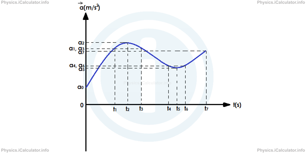
Thus, from t₀ to t₁ the acceleration is considered as increasing uniformly. Therefore, the average acceleration in this part of the graph is

< a⃗_{0 - 1} > = a⃗₀ + a⃗₁/2

The acceleration in t₁ and t₃ is numerically equal where it takes the maximum value of this interval at t₂. Therefore, we can write

< a⃗_{1 - 3} > = a⃗₁ + a⃗₂/2

From t₃ to t₄ the acceleration is considered as decreasing uniformly. Therefore, the average acceleration in this part of the graph is

< a⃗_{3 - 4} > = a⃗₃ + a⃗₄/2

Again, the acceleration in t₄ and t₆ is numerically equal where it takes the maximum value of this interval at t₅. Therefore, we can write

< a⃗_{4 - 6} > a⃗₄ + a⃗₅/2

Finally, from t₆ to t₇ the acceleration is considered again as increasing uniformly. Therefore, the average acceleration in this part of the graph is

< a⃗_{6 - 7} > a⃗₆ + a⃗₇/2

In this way, it was made possible to use the kinematic formulae in each interval separately in order to calculate the other quantities such as velocity and displacement.

Example 4

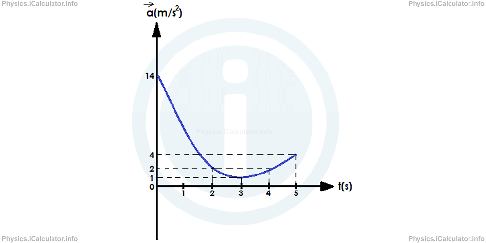
Calculate the total displacement for the motion described in the graph below if initially the object was moving at 20 m/s.

Solution

During the first two seconds, the object's acceleration decreases uniformly. Therefore, we can write for the average acceleration in this interval

< a⃗₁ > = < a⃗(0 - 2s) > = a⃗(2) + a⃗(0)/2
= 2 + 14/2
= 8 m/s²

Therefore, the displacement in this interval is

∆x⃗₁ = v⃗₀ × ∆t₁ + < a⃗₁ > × ∆t²₁/2
= 20 × 2 + 8 × 2²/2
= 40m + 16m
= 56m

We can find the velocity v⃗₁ at the end of the first interval, as we will use it in the other interval as well. Thus,

v⃗₁ = v⃗₀ + < a⃗₁ > × ∆t₁
= 20 + 8 × 2
= 36 m/s

Since the acceleration in t₁ = 2s is equal to that in t₃ = 4 s where the minimum acceleration is at t₂ = 3s, we have for the average acceleration during the second interval Δt₂:

< a⃗₂ > = < a⃗(2s - 4s) >
= a⃗(2) + a⃗(3)/2
= 2 + 1/2
= 1.5 m/s²

The displacement in this interval is

∆x⃗₂ = v⃗₁ × ∆t₂ + < a⃗₂ > × ∆t²₂/2
= 36 × 2 + 1.5 × 2²/2
= 72m + 3m
= 75m

The velocity v⃗₂ at the end of this interval is

v⃗₂ = v⃗₁ + < a⃗₂ > × ∆t₂
= 36 + 1.5 × 2
= 39 m/s

In the third interval (during the last second), the acceleration increases uniformly. Therefore, we can write

< a⃗₃ > = < a⃗(4s - 5s)>
= a⃗(4) + a⃗(5)/2
= 2 + 4/2
= 3 m/s²

The displacement in the last interval is

∆x⃗₃ = v⃗₂ × ∆t₃ + < a⃗₃ > × ∆t²₃/2
= 39 × 1 + 3 × 1²/2
= 40.5m

Hence, the total displacement is

∆x⃗_tot = ∆x⃗₁ + ∆x⃗₂ + ∆x⃗₃
= 56m + 75m + 40.5m
= 171.5m

The scheme below shows the relationship between the quantities involved in motion graphs:

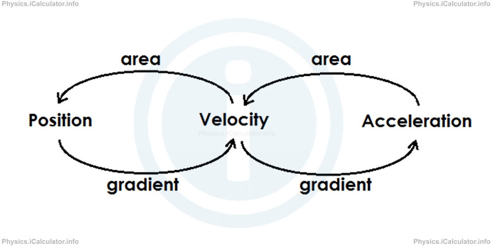
The interpretation of this scheme is as follows:

The gradient of the position vs time graph gives the velocity
The gradient of the velocity vs time graph gives the acceleration
The area under (above when negative) the velocity vs time graph gives the change in position (displacement)
The area under (above when negative) the acceleration vs time graph gives the change in velocity

You have reach the end of Physics lesson 3.11.5 What happens if the acceleration is not constant?. There are 5 lessons in this physics tutorial covering Acceleration v's Time Graph, you can access all the lessons from this tutorial below.

More Acceleration v's Time Graph Lessons and Learning Resources

Kinematics Learning Material
Tutorial ID	Physics Tutorial Title	Revision Notes	Revision Questions
3.11	Acceleration v's Time Graph
Lesson ID	Physics Lesson Title	Lesson	Video Lesson
3.11.1	Acceleration verse Time graph in Uniform motion
3.11.2	Acceleration verse Time graph in the uniformly accelerated (decelerated) motion
3.11.3	Why we cannot use the concept of Scalar Acceleration
3.11.4	Vector acceleration verse time graph and the hypothetical corresponding scalar acceleration vs time graph for the same motion
3.11.5	What happens if the acceleration is not constant?

Whats next?

Enjoy the "What happens if the acceleration is not constant?" physics lesson? People who liked the "Acceleration v's Time Graph lesson found the following resources useful:

Constant Feedback. Helps other - Leave a rating for this constant (see below)
Kinematics Physics tutorial: Acceleration v's Time Graph. Read the Acceleration v's Time Graph physics tutorial and build your physics knowledge of Kinematics
Kinematics Revision Notes: Acceleration v's Time Graph. Print the notes so you can revise the key points covered in the physics tutorial for Acceleration v's Time Graph
Kinematics Practice Questions: Acceleration v's Time Graph. Test and improve your knowledge of Acceleration v's Time Graph with example questins and answers
Check your calculations for Kinematics questions with our excellent Kinematics calculators which contain full equations and calculations clearly displayed line by line. See the Kinematics Calculators by iCalculator™ below.
Continuing learning kinematics - read our next physics tutorial: Motion in Two Dimensions. Projectile Motion

Help others Learning Physics just like you